


.
livello difficile
.
ARGOMENTO: BIOLOGIA E ECOLOGIA
PERIODO: XXI
AREA: CETACEI
parole chiave: Ziphius cavirostris
Key Oceanographic Characteristics of Cuviers Beaked Whale (Ziphius cavirostris): Habitat in the Gulf of Genoa (Ligurian Sea, NW Mediterranean)
Authors : Lanfredi C 1* , Azzellino A 1 , D’Amico A 2 , L Centurions 3 , Rella MA 4 , Pavan G 5 and M Podesta 6
| 1 Politecnico di Milano, SAY Environmental Engineering Division, University of Technology, Milan, Italy 2 Cubic Global Defence Inc., 2280 Historic Decatur Rd. 200, San Diego, CA, USA SCRIPPS, Scripps Institution of Oceanography, Climate, Atmospheric Science and Physical Oceanography, La Jolla, CA, USA 4 Engineering Department, CMRE Centre for Maritime Research and Experimentation, La Spezia, Italy 5 Department of Earth and Environment Science, Interdisciplinary Center CIBRA Bioacustica and Environmental Research, University of Pavia, Pavia, Italy 6 Museum of Natural History of Milan, Milano, Italy |
Copyright: © 2016 Lanfredi C, et al. This is an open-access article distributed under the terms of the Creative Commons Attribution License, which permits unrestricted use, distribution, and reproduction in any medium, provided the original author and source are credited.
| Corresponding Author: Lanfredi Caterina, Politecnico di Milano, University of Technology – SAY Environmental Engineering Division, Milan, Italy Tel: + 39-02-23996431 – Email: caterina.lanfredi@polimi.it Citation: Lanfredi C, Azzellino A, D’Amico A, Centurioni L, Rella MA, et al. (2016) Key Oceanographic Characteristics of Cuvier’s Beaked Whale (Ziphius cavirostris). Habitat in the Gulf of Genoa (Ligurian Sea, NW Mediterranean). J Oceanogr Mar Res 4:145. |

Zifio © S.Airoldi di Tethys Cuvier’s beaked whales – Tethys Research Institute
Abstract
Cuvier’s beaked whale presence has been associated worldwide with continental slope and submarine canyons areas. In the Mediterranean Sea, a hot spot of the species presence has been identified in the Genoa Canyon area, located in the Gulf of Genova (Ligurian Sea, NW Mediterranean Sea). Within the framework of the NATO Marine Mammal Risk Mitigation Project, several research cruises have been conducted between 1999 and 2011 in the Ligurian Sea area. During these cruises depth profiles of temperature, salinity, sound velocity, dissolved oxygen, fluorescence and turbidity as a function of depth were collected using a Conductivity, Temperature, Depth (CTD) and auxiliary sensors installed on a Rosette frame. Concurrently, Cuvier’s beaked whale (Ziphius cavirostris) presence was assessed through visual observations. The aim of this study was to investigate the environmental characteristics of a beaked whale habitat in the Genoa canyon area correlating beaked whale presence with the oceanographic variables. A Logistic Regression model was developed using the data collected during the oceanographic campaign carried out in summer 2002. Model accuracy was also evaluated in the same area based on the data collected 9 years later in summer 2011. The depth of the maximum dissolved oxygen (Depth Ox Max) turned out to be a significant predictor of beaked whale presence in the studied area. Higher presence probabilities of beaked whales were found associated to higher turbidities of deep-water layers in both the calibration and evaluation set. Results suggest dynamic predictors may act as proxy of macro-scale features that characterise beaked whale habitats. Particularly the depth the maximum oxygen concentration may be a tracer of the vertical exchanges of water masses (i.e., downwelling), transferring energy from the surface waters to the deep waters where beaked whales feed on their prey.
Introduction
The known sensitivity of beaked whales to anthropogenic sounds emissions [1–5] has stimulated worldwide the interest about the ecology of this species. A key element in the success of managing species of conservation concern is the knowledge of the species’ habitat use and preferences. Knowledge on the habitat use and preferences of beaked whales has been acquired worldwide in the last twenty years [6–13]. Several studies have reported a strong relationship with the topographic features of the sea bottom as animals were regularly observed over the continental slope in waters up to 2000 m of depth [11,14–16] and near submarine canyons [17]. Very few of these studies [10,17] have considered habitat predictors other than topographic or remote sensed parameters. Cuvier’s beaked whale (Ziphius cavirostris, G. Cuvier, 1823), is the only beaked whale regularly inhabiting the Mediterranean Sea area, where this species has been found associated with continental slope and with submarine canyons and seamounts areas [18–28]. In particular, the Genoa canyon area, located in the Ligurian sea (north western Mediterranean Sea), has been identified as a key habitat for Cuvier’s beaked whales [13].
Submarine canyons represent heterogeneous environments not only for their complex topography, but also for the fact that they are characterized by peculiar patterns of hydrography, flow sediment transport and accumulation [29]. Physical conditions in canyons are in fact often distinct from the surrounding shelf and slope, and can affect the structure of canyon communities [30]. Physical oceanographic conditions inside canyons, such as accelerated currents, upwelling and dense-water cascades, are often caused by topographic and climate forcing. These phenomena can be responsible for increasing suspended particulate matter concentrations and transport of organic matter from coastal zones to the deep ocean, enhancing both pelagic and benthic productivity inside canyon habitats [31]. Consequently, ocean dynamics may affect the distribution and behaviour of Cuvier’s beaked whales and the organisms forming the food web upon which the whales feed, through mechanisms such as concentration of nutrients and increase of primary production or aggregation of biomass due to convergence of water masses [9,31–33]. The opportunity to investigate how ocean dynamics influence the habitat selection of deep diving species is often limited by the availability of systematic oceanographic data collected in concurrence with marine mammal surveys. However, by collecting detailed oceanographic data, it is possible to identify additional key habitat characteristics. The aim of this study is therefore to correlate Cuvier’s beaked whale presence to the in situoceanographic measurements collected to a depth of about 1200 m during two dedicated research cruises conducted in 2002 and 2011 in the Genoa canyon area. This is the first time that measured oceanographic data are employed to model beaked whale habitat in the Mediterranean Sea. The specific objectives of this study are: 1) To evaluate whether dynamic parameters (i.e., temperature, salinity, sound velocity, dissolved oxygen, fluorescence and turbidity) may be used as potential predictors of the Cuvier’s beaked whale habitat; 2) To validate the prediction accuracy of the oceanographic-based models on an independent dataset collected in the same area; and 3) To improve the understanding of beaked whale key habitats characteristics in the Genoa canyon area.
Materials and Methods
Study area
The Gulf of Genoa (Figure 1) is located in north-western portion of the Ligurian Sea and is contained within the “International Sanctuary for the Protection of Mediterranean Marine Mammals’’ also known as “Pelagos Sanctuary”. Several canyons characterize the Gulf of Genoa with very steep slope gradients extending from the shelf break to a depth of about 2000 m. The Genoa canyon is the largest and the most northern canyon of the western Mediterranean Sea. Genoa canyon has its axis oriented northeast–southwest, with its two main canyons, the Polcevera and Bisagno, found in the head. These two canyons exhibit a linear along-axis topographic V shaped profile, are more than 700 m deep, 20 km wide and about are 60 km in length. Their steep walls suggest they are strongly affected by land sliding processes [34]. Directly east of this region is a wider canyon with a wide shelf to its south. The western part of the valley has a steep slope and several small canyons cut it. To the southwest, the canyon system descends into a deep abyssal plain. This large submarine valley (hereafter called “Genoa canyon area”) forms a boundary for the predominant circulation [35]. The circulation in the Ligurian basin consists of a basin-wide cyclonic gyre [36,37], which extends over the upper 500 m and can spread out to the west in to the Catalan Sea.

Figure 1: a) The Gulf of Genoa study area. b) Western Mediterranean Sea: Pelagos Sanctuary 638 borders (thick black lines) are shown.
Two major northward-flowing currents influence the general circulation in the basin: The Eastern Corsican Current that brings Tyrrhenian water in to the Ligurian Sea through the Corsica Channel and the Western Corsican Current which is part of the large cyclonic circulation. When these water masses join together north of Corsica, they form the Northern Current, also called the Liguro-Provencal- Catalan Current, which flows along the slope of the Italian, French and Spanish coasts [38]. A frontal region is commonly found at the limit of the cold core of the cyclonic Ligurian Sea circulation that separates the warmer, less saline peripheral zone near the coast from the denser and colder water in the central zone of the Ligurian Sea [39–41]. The occurrence of this permanent frontal area leads to an upwelling of deeper waters in the central zone and downwelling along the peripheral zone [39]. The upwelling provides the surface layer with inorganic nutrients that support a spring primary production which is higher than the average for the western Mediterranean waters and allows the fresh organic material produced near the surface to sink to the depths, enriching the entire water column and enhancing biological processes [40,35]. The Gulf of Genoa is north of the frontal area, however, the distribution of autotrophic biomass suggests an enriched zone in the southern part of the study area [35].
Data collection
From 1999 to 2011, more than 10 large-scale interdisciplinary sea trials were conducted in the Mediterranean Sea under the framework of the NATO Undersea Research Center (NURC)1 Marine Mammal Risk Mitigation Project (hereinafter called MMRM). This long-term study was designed to better understand the distribution of the cetacean population in the Mediterranean Sea, to develop analytical models to predict species presence and to test and improve passive acoustic monitoring methods. The majority of the at sea campaigns, entitled SIRENA, were conducted in the Ligurian Sea area. In this study data collected from the – in the Genoa canyon area in summer 2002 (SIRENA02/phase B) and 2011 (SIRENA 11/phase A) are analysed. Among the different sea trials conducted in the Ligurian Sea, these two campaigns were selected for the analysis because the sampling station protocol, oceanographic stations locations and time period were considered comparable.
Survey details of dataset used in the analysis are summarized in Table 1. The 2002 set has been used to construct the Cuvier’s beaked whale presence/absence model while the 2011 data set is used as independent evaluation set.
| Research cruise | SIREN 02 / phase B | SIREN 11 / phase A |
| Cruise Time Period | 5-23 July | 22 July-1 August |
| Research Vessels | NRV Alliance | NRV Alliance |
| Positive Effort *(km) | 323 | 870 |
| CTD stations | 21 | 18 |
| BW sightings | 24 | 14 |
Table 1: Summary of the data collected during research cruises SIRENA 02 (calibration set) and SIRENA 11 (evaluation set). *Km conducted with 4 visual observers and Beaufort sea state less than 4.
SIRENA ‘02/ phase2 was conducted in July 2002 covering an area of about 11,000 km2 (see Figure 2a). Oceanographic measurements were taken from the surface to a maximum depth of 1500 m, using a Conductivity, Temperature, Depth (CTD, Sea-Bird 911) and auxiliary sensors installed on a Rosette frame deployed from the N R/V Alliance at 21 pre-defined stations (Figure 1a). At each station, the following oceanographic data were collected: conductivity (mS/cm) to determine salinity, temperature (°C), density (kg/m3) derived from temperature and salinity, pressure to determine depth at which measurements are taken, fluorescence (ug/l) as a proxy for chlorophyll-a, dissolved oxygen (ml/l), turbidity an optical parameter collected with a turbidimeter as indicator of the scattered light due to suspended particles (FTU, formazine turbidity unit) and finally sound velocity (m/s) computed from salinity, temperature and depth measurements.

Figure 2a: SIRENA 02 dataset. Ziphius cavirostris sightings CTD stations and the corresponding 641 stations number are shown.
Cetacean visual sightings were collected using two big-eye verticalscale binoculars (Fujinon, 25*150, MTSX, field of view 2.75) mounted on the flying bridge of the NRV Alliance (at a height of 16 m above sea level) on the forward port and starboard sides while the ship was transiting at an average speed of 5-6 knots (i.e., about 10-12 km/h) in sea state conditions corresponding to a Beaufort scale lower than 4. Cetacean sightings were collected during daylight hours by a team of experienced observers that rotated through three observation positions (port, center, and starboard) and a recording position. Observers scanned the sea surface from 90° port to 90° starboard, where 0° is on the track line, with big-eye or regular binoculars (Fujinon 7*50 FMT/MT Field of view 7°30’). For every species encountered, time, bearing, radial distance, species, group size, behaviour, sighting cue, and swimming orientation (aspect) data were recorded. Environmental data, including sea state and effort status, were recorded every 30 minutes or more frequently if changes in conditions occurred. All the visual sighting data were recorded through dedicated data logging software. In the Genoa Canyon area a total of about 323 kilometres (174 nm) of track were surveyed under positive conditions (i.e., visual team on effort and Beaufort sea state lower than 4) and 24 sightings of Cuvier’s beaked whale were made.
The SIRENA11/phase A trial was conducted in 2011 during the time period and in the same area (Figure 2b and Table 1) investigated in 2002 and by used the same methods and protocols employed during SIRENA02 trial. Line transect surveys were conducted using passive acoustic and visual methods to determine the presence and absence of cetaceans. However, in the study presented here, only the visual data collected were employed in the validation model process to allow a comparison with the sea trial conducted in 2002. A total of about 870 km (470 nm) were covered in positive conditions resulting in 14 beaked whale sightings (i.e., 13 Cuvier’s beaked whales, and 1 undetermined beaked whale).

Figure 2b: SIRENA 11 dataset. Ziphius cavirostris sightings CTD stations and the corresponding
During the same time period, oceanographic data were collected at 18 stations for the same variables that were collected in 2002.
CTD Data Processing
Oceanographic measurements collected during the two research campaigns were calibrated and processed by NURC. The variables considered in this study were conductivity, temperature, salinity, density, dissolved oxygen, fluorescence, turbidity and sound velocity. Supplementary Figures S1 and S2 in Annex A shows the vertical profile of each of these variables as a function of depth for both SIRENA cruises. To better understand the spatial pattern of the studied variables a series of plots, cross-sectional to the canyon area, were developed following the orientation northeast–southwest of canyons main axis. Additional east–west section plots were produced (see Supplementary Figures S3-S7 for oxygen section plots only). For the SIRENA 02 calibration dataset 39 water column statistics were computed, station by station, based on the 8 oceanographic variables available: (conductivity (mS/cm), salinity (PSU), density (kg/m3), temperature (C°), fluorescence (μg/l), dissolved oxygen (ml/l), turbidity (FTU) and sound velocity (m/s)).
Table 3 summarizes the oceanographic variables derived from the CTD data used in the analysis. Minimum and maximum values (Min, Max) and the corresponding depths (Depth min, Depth max) were computed for every variable. Concerning the turbidity profiles the average (mean), median and standard deviation (SD) values were calculated. Gradients were computed as the ratio between the difference of the maximum and minimum values and the difference between the corresponding depths [i.e., (Max-Min)/(Depth Max-Depth Min)]. In addition, for the dissolved oxygen, the upper gradient (Ox Up gradient) was computed as the ratio between the difference of maximum and surface dissolved oxygen values and the depth of the maximum dissolved oxygen [i.e., (Max Ox-Ox at the Surface/Depth max)]. Fluorescence at 200 m was selected as the minimum measured fluorescence value. The depth of the 13.8°C isotherm was selected as the base of the thermocline. A Principal Component Analysis (PCA) was applied to the 39 parameters dataset to reduce the dimensionality of the CTD data matrix, and to select the most representative features of the water column profiles. For a better interpretation of the reduced components, the principal components previously extracted, were rotated applying a Varimax rotation criterion (i.e., the PCA solution was turned into a Factor Analysis solution), maintaining their orthogonality (i.e., the factors being still uncorrelated). By looking at the factor loadings matrix (i.e., the correlations of the original variables with the extracted factors) the most meaningful parameters within each factors were identified. Parameters lying on the same factor share the same information. The number of factors to retain was chosen on the basis of the “eigenvalue higher than 1” criterion (i.e., only the factors explaining more than the variance of one of the original variables were retained).
Data Preparation for the Regression Analysis: Sirena 02 dataset
The Genoa canyon area was divided into 308 cells of about 5 × 4 km by means of GIS Spatial Analyst tool. Visual effort was evaluated in terms of kilometres of track line per cell unit. Only the sightings reported on-effort and in favourable conditions were considered. Encounter rates were then calculated for each cell unit as the number of sightings per kilometre surveyed under favourable conditions.
To test whether cells were spatially auto-correlated, the Moran’s Index of the cell encounter rates was computed. According to Legendre et al. [42] the presence of spatial correlation may bias tests of significance for correlation or regression, when both the animal response variable and the environmental predictor are spatially autocorrelated. Moran’s Index provided an assessment that ensured the chosen grid size was large enough to have the cell units encounter rates not spatially correlated. The factors extracted through the PCA/FA analysis of the CTD data were used to describe the hydrological characteristics of the cells. Factor values, available as point observations at the stations, were interpolated by using an Inverse Distance Weighted algorithm (IDW2) [43] allowing attribution of the CTD factor values to every cell unit. The cell mean values of every CTD factor, were used as covariates in a subsequent regression analysis.
Regression analysis
Binary logistic regression analysis [44,45] was employed to correlate the beaked whales presence/absence data to the oceanographic predictors. Initially the cell means, calculated for every CTD factor were used as covariates. Afterwards, a new regression analysis was carried out, substituting the factor values with the most representative (i.e., the variables with the highest factor loadings) CTD parameters. To balance the number of absence observations, presence data were weighted on the basis of encounter rates, according to Azzellino et al. [24,25]. In order to select the best set of predictors, a forward stepwise method based on the significance of the Wald statistic [46] was used. Each predictor was tested for entry into the model one by one, based on the significance level of the Wald statistic. After each entry, variables that were already in the model were also tested for possible removal. The variable with the largest probability greater than the specified threshold value was removed, and the model re-estimated; the procedure stopped when no more variables met the entry or removal criteria or when the current model was the same as the previous. The classification performance of the logistic models was evaluated in terms of confusion matrices [47]. The threshold value (i.e., cut-off) for the presence classification was set at a 0.5 probability.
Model validation: Sirena 11 datasets
Predictions for the Genoa canyon area were made using the habitat model developed on the 2002 data set (evaluation set). Model validation was then conducted using as independent evaluation set the data collected in the 2011 campaign and by evaluating the agreement between predictions and actual observations. A 2×2 cross tabulation was created between observed and predicted presence/absence data (i.e., the confusion matrix according to Kohavi and Provost [47]). The confusion matrix can be used to describe predictive performance of models [47,48]. The sensitivity (i.e., the true positive fraction, the proportion of the positive observations in agreement with the presence predictions over the total positive observations) was used to evaluate the accuracy and the reliability of the models. For the validation set a more conservative threshold value, set at a 0.75 probability, was assumed for the presence prediction.
Results
PCA / FA of CTD data.
As shown in Table 2, the 91% of the original variance was summarized by 8 factors, retained on the basis of the “eigenvalue higher than 1” criterion.
| Initial Eigen values | Rotation Sums of Squared Loadings | |||||
| Component | Total | % of Variance | Cumulative % | Total | % of Variance | Cumulative % |
| 1 | 12,289 | 31511 | 31511 | 10,054 | 25,779 | 25,779 |
| 2 | 9,468 | 24,277 | 55788 | 8,168 | 20,943 | 46,722 |
| 3 | 4,078 | 10,457 | 66,245 | 6,170 | 15,819 | 62541 |
| 4 | 3,219 | 8,253 | 74498 | 3,047 | 7,813 | 70354 |
| 5 | 2,217 | 5,684 | 80181 | 2,402 | 6,159 | 76513 |
| 6 | 1,684 | 4,319 | 84,500 | 2,286 | 5,863 | 82375 |
| 7 | 1,438 | 3,688 | 88188 | 1,834 | 4,703 | 87078 |
| 8 | 1,131 | 2,900 | 91088 | 1,564 | 4,010 | 91088 |
Table 2: Initial eigenvalues, variance explained, and cumulative variance explained for the principal component analysis (PCA) solution and the factor analysis (FA) rotated solution.
These 8 factors were interpreted on the basis of the factor loadings (Table 3) as follows:
| Factors | |||||||||
| Variables | F1 | F2 | F3 | F4 | F5 | F6 | F7 | F8 | |
| 1 | Min Conduct | -0049 | 0921 | -0040 | 0150 | 0093 | -0215 | 0048 | 0038 |
| 2 | Max Conduct | 0223 | -0060 | 0958 | 0109 | 0056 | -0033 | 0028 | -0019 |
| 3 | Conduct gradient | 0224 | -0265 | 0927 | 0071 | 0032 | 0017 | 0016 | -0027 |
| 4 | Min Temp | -0630 | 0568 | -0164 | -0.005 | -0078 | -0167 | 0037 | 0176 |
| 5 | Max Temp | 0273 | 0149 | 0929 | 0090 | 0060 | -0032 | -0077 | 0027 |
| 6 | Temp gradient | 0375 | 0035 | 0908 | 0086 | 0071 | 0001 | -0080 | -0007 |
| 7 | Depth 13.8° | 0139 | 0892 | -0039 | 0138 | 0157 | -0280 | -0105 | -0.025 |
| 8 | Min Fluoresc | -0946 | 0056 | -0182 | -0011 | -0047 | 0042 | 0058 | -0006 |
| 9 | Fluoresc at surf | -0108 | -0336 | 0001 | -0313 | -0493 | 0385 | -0218 | 0019 |
| 10 | Max Fluoresc | 0051 | -0719 | 0202 | -0.003 | 0385 | 0187 | -0197 | -0306 |
| 11 | Fluoresc 200m | -0975 | 0092 | -0164 | -0066 | -0040 | 0000 | -0024 | -0007 |
| 12 | Depth Fluoresc max | 0125 | 0877 | 0007 | 0190 | 0153 | 0143 | 0148 | 0203 |
| 13 | Fluoresc gradient | 0096 | -0716 | 0209 | -0.003 | 0384 | 0183 | -0199 | -0303 |
| 14 | Min Oxygen | -0985 | 0049 | -0104 | -0055 | 0018 | 0014 | -0037 | -0017 |
| 15 | Max Oxygen | 0132 | -0852 | 0363 | -0163 | 0154 | 0054 | 0022 | 0004 |
| 16 | Ox at the surf | -0124 | -0223 | -0022 | 0041 | 0001 | 0934 | -0.030 | -0032 |
| 17 | Depth Ox min | 0774 | 0534 | 0180 | 0030 | 0054 | -0126 | -0108 | -0.002 |
| 18 | Depth Ox max | -0088 | 0035 | 0072 | 0060 | -0078 | 0139 | 0834 | 0026 |
| 19 | OxUp gradient | 0159 | 0109 | 0033 | -0104 | 0041 | -0931 | -0201 | 0057 |
| 20 | Oxygen gradient | -0916 | -0312 | -0184 | -0060 | -0023 | 0104 | 0037 | -0.002 |
| 21 | Min Density | -0.083 | -0338 | -0571 | 0088 | 0499 | 0031 | 0377 | -0156 |
| 22 | Max Density | 0977 | -0044 | 0173 | 0063 | 0033 | -0044 | 0023 | 0018 |
| 23 | Depth Density max | 0584 | -0436 | 0340 | -0203 | 0261 | 0122 | -0045 | -0332 |
| 24 | Density gradient | -0973 | 0103 | -0170 | -0.030 | -0080 | 0025 | -0.030 | 0022 |
| 25 | Min Salinity | 0056 | -0106 | 0283 | 0138 | 0747 | -0090 | -0326 | -0166 |
| 26 | Max Salinity | 0974 | -0033 | 0158 | -0020 | 0012 | -0071 | 0053 | 0044 |
| 27 | Depth Salinity min | 0328 | 0306 | 0190 | -0037 | 0671 | 0040 | 0178 | 0208 |
| 28 | Depth Salinity max | 0826 | 0395 | -0.005 | 0150 | 0005 | -0126 | -0116 | 0039 |
| 29 | Salinity gradient | -0883 | -0094 | -0205 | -0176 | -0290 | 0102 | 0174 | 0054 |
| 30 | Min Turbidity | 0053 | 0187 | -0207 | -0197 | -0012 | -0059 | 0037 | 0879 |
| 31 | Max Turbidity | 0126 | -0532 | -0255 | 0507 | 0380 | 0064 | -0147 | 0135 |
| 32 | Turbidity mean | 0135 | 0415 | 0118 | 0839 | -0043 | 0023 | 0138 | -0095 |
| 33 | Turbidity median | 0072 | 0450 | 0080 | 0806 | -0085 | 0030 | 0155 | -0188 |
| 34 | Turbidity SD | 0124 | 0044 | 0008 | 0936 | 0203 | 0070 | 0043 | -0006 |
| 35 | Sound speed min | 0100 | 0947 | -0035 | 0206 | 0068 | -0048 | 0031 | 0027 |
| 36 | Sound speed max | 0168 | -0172 | 0898 | -0112 | 0154 | -0007 | -0012 | -0265 |
| 37 | Depth sound speed min | -0014 | 0308 | -0262 | 0194 | 0066 | -0040 | 0689 | 0021 |
| 38 | Depth sound speed max | -0287 | -0683 | -0065 | 0097 | -0304 | -0167 | -0169 | 0348 |
| 39 | Sound speed gradient | 0110 | -0486 | 0.790 | -0170 | 0109 | 0011 | -0022 | -0240 |
| % of Variance | 250.78 | 200.94 | 150.82 | 70813 | 60159 | 50,863 | 40,703 | 40.01 | |
| Cumulative % | 250.78 | 460.72 | 620.54 | 700.35 | 760.51 | 820.38 | 870.08 | 910.09 | |
Table 3: Factor analysis matrix with the variables used in the analysis. Each Factor loading represents the correlation between the original variables and the factor. Higher correlation coefficients are presented in bold.
Factor 1 (F1) is positively correlated with the maximum values of density, salinity, and with depth of the maximum salinity and minimum dissolved oxygen. F1 is also inversely correlated with the minimum measured fluorescence value (at a depth of about 200 m), and with the gradients of density and salinity. It accounts for 25.78% of the total variance.
Factor 2 (F2) is directly correlated with the minimum values of conductivity, sound velocity and temperature (13.8 °C) and with the depth of the maximum fluorescence. F2 is also inversely correlated with maximum values of dissolved oxygen and fluorescence. F2 accounts for 20.9% of the total variance.
Factor 3 (F3) is correlated with the maximum values of temperature, conductivity and sound velocity, close to the surface. F3 accounts for 15.8% of the total variance.
Factor 4 (F4) is the directly correlated with the mean, median and SD values of the turbidity. F4 accounts for 7.8% of the total variance.
Factor 5 (F5) is positively correlated with minimum salinity and the depth of the minimum salinity. It accounts for 6% of the total variance.
Factor 6 (F6) is positively correlated with dissolved oxygen surface values and inversely correlated with the oxygen upper gradient. F6 accounts for 5.8% of the total variance.
Factor 7 (F7) is positively correlated with the depth of maximum oxygen and the depth of the minimum sound speed. F7 accounts for 4.7% of the variance.
Factor 8 (F8) positively correlated with the minimum turbidity values, F8 accounts for 4% of the variance.
As described, the data available from the 21 CTD stations were interpolated through a IDW algorithm to a grid of 486 cells of about 3 nautical miles (0.05°) of cell size. Moran’s Index tested on the Cuvier’s beaked whale encounter rate showed that cells were not spatially auto correlated (Moran coefficient: I: 0.133962; SD: 0.032712).
Model Development: Sirena 02 Dataset
The 8 factors were evaluated as predictors through the logistic regression analysis. The cell mean values, calculated for every factor, were used as covariates in the models. The stepwise procedure selected “Factor 7” (i.e., water column oxygen feature) as the best predictor (see Table 4). As shown in Table 5 the model showed a good accuracy in predicting both presence and absence cells (72.2%).
| 95.0% C.I. for EXP(B) | ||||||||
| B | S.E. | Forest | df | Sig. | Exp(B) | Lower | Upper | |
| Step 1 | Factor 7 1,779 | 0724 | 6,044 | 1 | 00:01 | 5,926 | 1,434 | 24482 |
| Constant-0,282 | 0.389 | 0528 | 1 | 0467 | 0754 | – | – | |
Table 4: Results of the binary logistic regression analysis model in the calibration set (SIRENA 02). Presence/absence of Cuvier’s beaked whale were correlated with cell means, calculated for every factor. The following statistics are shown: B: Unstandardized regression coefficient; S.E.: Standard error of B; Wald statistic for the included parameter; df: Degrees of freedom; P: Level of significance.
| Predicted Zc01* | |||||
| Absence | Presence | Percentage Correct | |||
| Step 1 | Observed Zc01* | Absence | 13 | 5 | 72.2 |
| – | Presence | 5 | 13 | 72.2 | |
| Overall Percentage | – | – | – | Overall Percentage | |
Table 5: Confusion matrix of the model using factors cell means as predictors (Table 4).*Zc01 indicate Cuvier’s Beaked whale presence (1) and absence (0) cells.
Afterwards, a new regression analysis was carried out by substituting the factor with the original variables having the highest factor loading on the selected factor. In this second regression, the depth (m) of the maximum oxygen, (factor loading: 0.879) and the depth (m) of the maximum sound speed (factor loading: 0.689) were used as covariates. The strongest predictor of Cuvier’s beaked whale presence was the depth of the maximum oxygen value (hereinafter called: “Depth Ox Max”) being directly correlated to the whale presence (Table 6). In this case the overall model accuracy was 61.1%, showing a higher accuracy for the presence cells (66.7%) than for the absence cells (55.6%) see Table 7. Basically, as shown in Figure 3, Cuvier’s beaked whale presence in the Genoa canyon area is associated with cells showing deeper maximum oxygen layer with respect to the absence cells where the maximum oxygen layer was shallower.
| 95.0% C.I.for EXP(B) | ||||||||
| B | S.E. | Forest | df | Sig. | Exp(B) | Lower | Upper | |
| Step 1 Depth Ox Max | 0449 | 0198 | 5,122 | 1 | 0024 | 1,567 | 1,062 | 2,312 |
| Constant | -17.47 | 7,724 | 5,114 | 1 | 00:24 | 0 | – | – |
Note: The following statistics are shown: B: Unstandardized regression coefficient; S.E.:Standard error of B; Wald statistic for the included parameter; df: Degrees of freedom; P: Level of significance.
Table 6:Results of the binary logistic regression analysis model performed in calibration set (SIRENA 02) using depth of the maximum oxygen value (Depth Ox max) as covariate.
| Predicted Zc01* | |||||
| Absence | Presence | Percentage Correct | |||
| Step 1 | Observed Zc01* | Absence | 10 | 8 | 55.6 |
| – | Presence | 6 | 12 | 66.7 | |
| Overall Percentage | – | – | – | 61.1 | |
Table 7: Confusion matrix of the models performed using depth of the maximum oxygen (Depth Ox Max) as predictor (Table 6).*Zc01 indicate Cuvier’s Beaked whale presence (1) and absence (1) cells.

Model Validation: Sirena 11 Dataset
For model validation, the maximum oxygen depths were calculated station by station from the CTD data collected during the SIRENA 11/ phase A campaign and interpolated by using the IDW algorithm to the same grid that was used for the 2002 analysis. Presence/absence predictions for the Genoa canyon area were made using the model based on the “Depth Ox Max” predictor developed on the 2002 data set (calibration set). Such predictions were overlaid to the Cuvier’s beaked whale observations collected during the Sirena 11/ phase A campaign (i.e., independent evaluation set) (Figure 4). The accuracy of the model was assessed through a cross-tabulation analysis (Tables 8). A Chi-square test showed a significant association between model prediction and the observations (χ2 = 4.267; df = 1; P-level < 0.05). The model showed good performance of classification, being slightly more accurate in classifying absence cells (87.5%) rather than presence cells (62.5%). This might be the effect of the low sample size (8 presence cells) used for the evaluation set.
| ZC predicted | |||||
| Absence cells | Presence cells | Correct prediction | |||
| Zc Observed | Absence cells | Count | 7 | 1 | 8 |
| – | % | 87.5 | 12.5 | 87.5 | |
| Presence cells | Count | 3 | 5 | 8 | |
| – | % | 37.5 | 62.5 | 62.5 | |
| Overall percentage | – | – | – | – | 75.0 |
Table 8: Cross-tabulation analysis of the model predictions versus the Cuvier’s beaked whale observations of the evaluation set (SIRENA 11).

Discussion
In this study, in situ oceanographic measurements collected in Genoa canyon area in concurrence with Cuvier’s beaked whale sightings, were analysed with the aim to identify the mechanisms that may influence the habitat selection of beaked whales at the canyon scale. This is the first time that measured oceanographic data were employed to model beaked whale presence in the Mediterranean Sea. The only other available example in the literature concerns the northern Adriatic Sea where CTD data were used to predict the habitat of common bottlenose dolphin, Tursiops truncatus [32]. In situ oceanographic measurements such as temperature and salinity were successfully employed to model beaked whale spatial density in the Pacific Ocean [10,49]. In that study the extent of the investigated spatial scale pointed out the effect of sea surface temperature and thermocline strength differences as boundary conditions. In the Ligurian Sea, the strong relationship of the species presence with the Genoa Canyon area [21,24–27] supports the hypothesis that this particular area has a special ecological meaning for Cuvier’s beaked whale, probably related to the prey availability within the canyon. In situ oceanographic measurements provided new elements for identifying the ecological mechanisms that can influence beaked whale habitat selection at canyon scale. The results of this study suggest that dynamic variables derived from oceanographic measurements (i.e., CTD data) may be employed as predictors of Cuvier’s beaked whale presence in Genoa canyon area. Particularly, the depth (m) of the maximum concentration of dissolved oxygen (Depth Ox Max) was found to be a significant predictor of beaked whale presence, providing good performance of presence/absence classification in the calibration dataset (SIRENA 02) and showing a good model accuracy for the evaluation set (SIRENA 11). The fact that model accuracies were comparable for both the calibration and evaluation data set proves the reliability of the predictor “Depth Ox Max” for the data collected 9 years apart. Higher probabilities of beaked whale presence are in fact directly associated with the areas showing the deepest maximum oxygen layer. Dissolved oxygen profiles for this region show that the maximum dissolved oxygen concentration occurs within the first 50 m of the water column, than it decreases with depth, the minimum concentration layer occurring around 400 m, and then showing a low and gradual increase in concentration up to the maximum recording depth (about 1200 m). It is widely known that beaked whales are deep diving species, performing deep foraging dives to feed on deep water food resources. Cuvier’s beaked whale diving profiles in the Ligurian Sea [50] showed foraging activity in mesopelagic to bathypelagic water depths (613–1297 m). The stomach contents of 3 Cuvier’s beaked whales stranded along the Ligurian coast consisted of digested mesopelagic cephalopod beaks principally of the Histioteuthidae family, specifically Histioteuthis reversa and H. bonnellii and other cephalopods species such as Octopoteuthis spp. (Octopoteuthidae), Galiteuthis armata (Cranchiidae), Chiroteuthis. veranii (Chiroteuthidae) e Ancistroteuhis lichtensteinii(Onychoteuthidae) [51]. From this perspective, the predictor “Depth Ox Max” selected in this study does not reflect the foraging depths generally used by the species, but may be reasonably considered a proxy for vertical exchanges in the water masses. In fact, dissolved oxygen in the ocean is known to be a useful tracer for tracking the movement of water-types and water-masses [52]. It is known that submarine canyons may modify flow, shelf-slope exchanges of water and material [53,54] and this combination may influence the transport of particulate organic matter that influence productivity. The degree of complexity of the sea bottom, relative position, size and morphology of the canyons as well as wind stress strength, affect the local circulation, altering current flows favouring the rise or sinking of the water masses [55,56]. In addition, canyons environments are interested by phenomena such as dense shelf water cascade that transport large amounts of water, sediment and organic matter, downslope in the canyon to the deep ocean, reshaping submarine canyon floors and affecting the deep-sea environment [57]. In the Genoa canyon area, a deeper maximum oxygen layer could suggests a sinking of productive surface waters that brings oxygenated waters deeper due to the motion of the water mass in the canyon (coastward downwelling) stimulated by the frontal area. This downwelling motion allows the fresh organic material produced near the surface to sink to depth, thus enriching the water column and enhancing the biological processes. It is widely accepted that vertical sinking of organic material is one of the main source of nutrients to the deep-sea floor [56]. The results obtained on seawater samples collected during SIRENA 02 [35] in the Genoa canyon, suggest that the transfer of organic matter to depth, driven by downwelling, may sustain intense microbial activity in the mesopelagic layer. Moreover, the same authors found increases in ectoenzymatic activity in the mesopelagic layer that was linked to the presence of active microbial assemblages which was thought to enhance the recycling potential of the food web. According to Misic and Fabiano [35] the productive events, that are not dependent on surface productivity processes, can be associated by increase of turbidity at depth. To investigate this aspect, the mean values of turbidity between the depths of 400 m and 1200 m (range of possible feeding habitat of beaked whale), were calculated in both calibration (SIRENA 02) and validation set (SIRENA 11). It was shown that the areas with higher presence probability (i.e., probability higher than 75% based on the Depth Ox max model predictions), are also characterised by a higher mean (Mann Whitney U = 2634; P-level < 0.1) and maximum (Mann Whitney U = 2401; P-level < 0.05) turbidity with respect to the lower probability areas (i.e., probability lower than 75% based on the Depth Ox max model predictions) as shown in Figure 5.
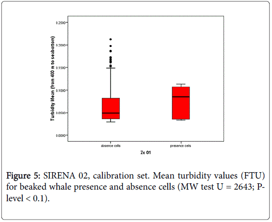
The same pattern was also observed in the evaluation set (Mann Whitney U = 9317; p-level < 0.05) (Figure 6). Thus, the depth of the maximum oxygen layer acts as a proxy for areas where vertical motions support the enhancing of biological processes at the different trophic levels. The trophic enrichment suggested by the increase of the turbidity in the canyon’s deep waters may be an attractor for beaked whale prey, such as the mesopelagic cephalopods, and be a key factor in the beaked whale habitat selection within the canyon.

Conclusion
This study provided the unique opportunity to investigate how ocean dynamics might influence the habitat selection of Cuvier’s beaked whale in one Mediterranean key habitat, the Genoa Canyon area. In situ oceanographic measurements were employed as predictors to model beaked whale presence in the Canyon area. The depth of the maximum oxygen was found directly correlated with beaked whale presence. The relevance of such predictor was also validated based on an independent dataset which was generated 9 years later in the same area. We assume that depth of the maximum oxygen might be a proxy of downwelling regions where energy from the richer surface waters is transferred to the deep waters, enhancing the productivity in the meso- and bathy-pelagic environment where beaked whales feed on their prey. These results suggest that dynamic predictors may act as proxy of the macro-scale features that characterise beaked whale habitat. Further research should be dedicated to identify more accessible (e.g. remote sensed parameters) proxies of such dynamics, enabling the confirmation of these results and improving the identification of beaked whales habitat in different areas of the Mediterranean Sea.
Acnowledgement
The authors acknowledge and appreciate the support of the NRV “Alliance’s” Captains and crew for their passionate support during the Sirena/MED trials. Additionally, the authors would like to acknowledge the MMRM Project, all NURC (CMRE) personnel that worked at the project during the years and all the colleagues from different research organization who participated in the data-collection effort. The authors want to thank Dr. James Eckman, for the support and interest demonstrated about the topic of this study, Jerry Olen of SPAWAR Systems Center Pacific for his continued support and Philippa Dell that reviewed the paper for English language. This work was principally supported by the Office of Naval Research (Grant N00014-10-1-0533) and also partially supported by the EC FP7 Marie Curie Actions People, Contract PIRSES-GA-2011-295162–ENVICOP project (Environmentally Friendly Coastal Protection in a Changing Climate).
1NURC, has recently changed name. Now is CMRE, Centre for Maritime Research and Experimentation.
2The IDW interpolator assumes that each input point has a local influence that diminishes with distance. So the points closer to the processing cell have greater weight than more distant points.
Copyright: © 2016 Lanfredi C, et al. This is an open-access article distributed under the terms of the Creative Commons Attribution License, which permits unrestricted use, distribution, and reproduction in any medium, provided the original author and source are credited.
Alcune delle foto presenti in questo blog possono essere state prese dal web, pur rispettando la netiquette, citandone ove possibile gli autori e/o le fonti. Se qualcuno desiderasse specificarne l’autore o rimuoverle, può scrivere a infoocean4future@gmail.com e provvederemo immediatamente alla correzione dell’articolo
PAGINA PRINCIPALE - HOME PAGE
References
- Simmonds MP, Lopez-Jurado LF (1991) Whales and the military. Nature 351: pp448.
- Frantzis A (1998) Does acoustic testing strand whales? Nature 392: 29.
- Jepson PD, Arbelo M, Deaville R, Patterson IAP, Castro P, et al. (2003) Gas bubble lesions in stranded cetaceans: was sonar responsible for a spate of whale deaths after an Atlantic military exercise? Nature 425: 575-576.
- Fernández A, Edwards JF, Rodríguea F, Espinosa de los Monteros A, Herráez P, et al. (2005) “Gas and fat embolic syndrome” involving a mass stranding of Beaked whales (family Ziphiidae) exposed to anthropogenic sonar signals. Vet Pathol 42: 446-457.
- Cox TM, Ragen TJ, Read AJ, Vos E, Baird RW, et al. (2006) Understanding the impacts of anthropogenic sound on beaked whales. J Cetacean Res Manage 7: 177-187.
- MacLeod CD (2000) Distribution of beaked whales of the genus Mesoplodon in the North Atlantic (Order: Cetacea, Family: Ziphiidae). Mammal Review 30: 1-8.
- Baumgartner MF, Mullin KD, May LN, Leming TD (2000) Cetaceans habitats in the northern Gulf of Mexico. Fish Bull 99: 219-239.
- Davis RW, Fargion GS, May N, Leming TD, Baumgartner MF (1998) Physical habitat of cetaceans along the continental slope in the north-central and western Gulf of Mexico Mar MammSci 14: 490-507.
- Davis RW, Ortega-Ortiz JG, Ribic CA, Evans WE, Biggs DC, et al. (2002) Cetacean habitat in the northern oceanic Gulf of Mexico. Deep Sea Res I 49: 121-142.
- Ferguson MC, Barlow J, Reilly SB,Gerrodette T (2006) Predicting Cuvier’s (Ziphiuscavirostris) and Mesopolodon beaked whale population density from habitat characteristics in the eastern tropical Pacific Ocean. J Cetacean Res Manage 7: 287-299.
- Waring GT, Hamazaki T, Sheenan D, Wood G, Baker S (2001) Characterization of beaked whale (Ziphiidae) and sperm whale (Physetermacrocephalus) summer habitat in shelf-edge and deeper waters off the northeast US. Mar MammSci 17: 703-17.
- MacLeod CD,D’Amico A (2006) A review of knowledge about behavior and ecology of beaked whales in relation to assessing and mitigating potential impacts from anthropogenic noise. J Cetacean Res Manage 7: 211-221.
- MacLeod CD, Mitchell G (2006) Known key areas for beaked whales around the world. J Cetacean Res Manage 7: 309-322.
- Hamazaky T (2002) Spatiotemporal prediction models of North Atlantic Ocean (from cape hatteras, North Carolina, U.S.A. to nova Scotia, Canada) cetacean habitats in the mid-western. Mar MammSci 18: 920-939.
- Hooker SK, Whitehead H, Gowans S, Baird RW (2002) Fluctuations in distribution and patterns of individual range use of northern bottlenose whales. Mar EcolProgSer 225: 287-297.
- MacLeod CD, Zuur AF (2005) Habitat utilisation by Blainville’s beaked whales off Great Abaco, Northern Bahamas, in relation to seabed topography. Mar Biol 147: 1-11.
- Wimmer T, Whitehead H (2004) Movements and distribution of northern bottlenose whales, Hyperoodonampullatus, on the Scotian Slope and in adjacent waters. Can J Zool 82: 1782-1794.
- Cañadas A, Sagarminaga R,García-Tiscar S (2002) Cetacean distribution related with depth and slope in the Mediterranean waters off southern Spain. Deep Sea Res I 49: 2053-2073.
- Cañadas A, Vazquez JA (2014) Conserving Cuvier’s beaked whales in the Alboran Sea (SW Mediterrranen): Identification of high density areas to be avoided by man-made sound. Bio Cons 178: 155-162.
- D’Amico A, Bergamasco A, Zanasca P, Carniel E, Portunato N, et al. (2003) Qualitative Correlation of Marine Mammals with Physical and Biological parameters in the Ligurian Sea. IEEE J Ocean Eng 28: 29-43.
- Moulins A, Rosso M, Nani B, Wurtz M (2007) Aspects of the distribution of Cuvier’s beaked whale (Ziphiuscavirostris) in relation to topographic features in the Pelagos Sanctua ry (north-western Mediterranean Sea). J Mar BiolAssoc UK 87: 177-186.
- Moulins A,Rosso M, Ballardini M, Wu¨rtz M (2008) Partitioning of the Pelagos Sanctuary (north-581 westernMediterranean Sea) into hotspots and coldspots of cetacean distributions. J Mar Biol Ass 88: 1273-1281.
- Gannier A,Epinat J (2008) Cuvier’s beaked whale distribution in the Mediterranean Sea: results from small boat surveys 1996–2007. J Mar BiolAssoc UK 88: 1245-1251.
- Azzellino A, Airoldi S, Gaspari S, Nani B (2008) Habitat use of cetaceans along the Continental Slope and adjacent waters in the Western Ligurian Sea. Deep Sea Res I, 55: 296-323.
- Azzellino A, Lanfredi C, D’Amico A, Pavan G, Podestà M, et al. (2011) Risk mapping for sensitive species to underwater anthropogenic sound emissions: model development and validation in two Mediterranean areas. Mar. Pollut Bull 63: 56-70.
- Azzellino A, Panigada S, Lanfredi C, Zanardelli M, Airoldi S, et al. (2012) Predictive Habitat Models For Managing Marine Areas: Spatial And Temporal Distribution Of Marine Mammals Within The Pelagos Sanctuary (Northwestern Mediterranean Sea). Ocean Coast Manag 67: 63-74.
- Tepsich P, Rosso M, Halpin PN, Moulins A (2014) Habitat preference of two deep diving cetacean species in the northern Ligurian Sea. Mar EcolProgSer 508: 247-260.
- Arcangeli A, Campana I, Marini L, MacLeod CD (2016) Long-term presence and habitat use of Cuvier’s beaked whale (Ziphiuscavirostris) in the Central Tyrrhenian Sea. Mar Ecol 37: 269-282.
- De Leo FC, Smith CR, Rowden AA, Bowden DA, Clark MR (2010) Submarine canyons: hotspots of benthic biomass and productivity in the deep sea. Proc R SocLond B BiolSci 277: 2783-2792.
- Vetter EW, Dayton PK (1999) Organic enrichment by macrophyte detritus, and abundance patterns of megafaunal populations in submarine canyons. Mar EcolProgSer 186: 137-148.
- Ainley DG, Jongsomjit D, Ballar G, Thiele D, Fraser WR, et al. (2012) Modeling the relationship of Antarctic minke whales to major ocean boundaries. Polar Biol 35: 281-290.
- Bearzi G, Azzellino A, Politi E, Costa M, Bastianini M (2008) Influence of seasonal forcing on habitat use by bottlenose dolphins Tursiopstruncatus in the northern Adriatic Sea. Ocean Sci J 43: 175-182.
- Tynan CT, Ainley DG, Barth JA, Cowles TJ, Pierce SD, et al. (2005) Cetacean distributions relative to ocean processes in the northern California Current System. Deep Sea Res II 52: 145-167.
- Mignon S, Cttaneo A, Hassoun V, Larroqu, C, Corradi N, et al. (2011) Morphology, distribution and origin of recent submarine landslides of the Ligurian Margin (North-western Mediterranean): some insights into geohazard assessment. Mar Geophys Res 32: 225-243.
- Misic C, Fabiano M (2006) Coenzymatic activity and its relationship to chlorophyll-a and bacteria in the Gulf of Genoa (Ligurian Sea, NM Mediterranean). J Marine Syst 60: 193-206.
- Ovchinnikov M (1966) Circulation in the surface and intermediate layers of the Mediterranean Oceanology 6: 48-59.
- Crépon M, Wald L, Monget JM (1982) Low-frequency waves in the Ligurian Sea during December 1977. J Geophys Res 87: 595-600.
- Millot C (1991) Mesoscale and seasonal variabilities of the circulation in the western Mediterranean. Dynam. Atmos Oceans 15: 179-214.
- Sournia A, Brylinsky JM, Dallot S, Le Corre P, M Leveau, Prieur L, et al. (1990) hydrological fronts off cotesfrancaises: sites workshops Frontal program OceanolActa 13: 413-438.
- Savenkoff C, Prieur L, Reys JP, Lefevre D, Dallot S, Deni S (1993) Deep microbial communities evidenced in the Liguro- Provencal front by their ETS activity. Deep Sea Res I 40: 709-725.
- Stemmann L, Prieur L, Legendre L, Taupier-Letage I, Picheral M, et al. (2008) Effects of frontal processes on marine aggregate dynamics and fluxes: An interannual study in a permanent geostrophic front (NW Mediterranean). J Marine Syst 70: 1-20.
- Legendre P, Dale MRT, Fortin MJ, Gurevitch J, Hohn M, et al. (2002) The consequences of spatial structure for the design and analysis of ecological field surveys. Ecography 25: 601-615.
- Webster R, Oliver MA (2007) Geostatistics for environmental science. John Wiley and Sons, LTD. Toronto, Canada, p: 271.
- Afifi A, Clark V (2003) Computer-Aided Multivariate Analysis. Texts in Statistical Science (4th edn.) Chapman & Hall/CRC Press,p: 512.
- Guisan A, Zimmermann NE (2000) Predictive habitat distribution models in ecology. Ecol Model 135: 147-186.
- Hosmer DW, Lemeshow S (2000) Applied logistic regression(2nd edn.) John Wiley & Sons, New York.
- Kohavi R, Provost F (1998) Glossary of terms. Machine Learning 30: 271-274.Pearce JL, Burgman MA, Franklin DC (1994) Habitat selection by helmeted honeyeaters. Wildl Res 21: 53-63.
- Forney K, Ferguson MC, Becker EA, Fiedler PC, Redfern JV, et al. (2012) Habitat-based spatial models of cetacean density in the eastern Pacific Ocean. Endang Species Res 16: 113-133.
- Tyack PL, Johnson M, Aguilar Soto N, Sturlese A, Madsen PT (2006) Extreme diving of beaked whales. J ExpBiol 209: 4238-4253.
- OrsiRelini L, Garibaldi F (2005) Mesopelagic cephalopods biodiversity in the Cetacean Sanctuary as a result of direct sampling and observations on the diet of the Cuvier’s Beaked whale, Ziphiuscavirostris. Biol Mar Medit 12: 106-115.
- Imasato N, Kobayashi T, Fujio S (2000) Study of water motion at the dissolved minimum layer and local oxygen consumption rate from the Lagrangian viewpoint. J Oceanogr 56: 361-377.
- Hickey BM (1995) Coastal Submarine Canyons. In: Müller P, HendersonD (eds.) Topographic effects in the Ocean, SOEST Special Publication, University of Hawaii, Manoa, pp: 95-110.
- Perenne N, Lavelle JW, Smith DC, Boyer DL (2001) Impulsively started flow in a submarine canyon: comparison of results from laboratory and numerical models. J Atmos Oceanic Technol 18: 1698-1718.
- Klinck JM (1996) Circulation near submarine canyons: a modeling study. J Geophys Res 101: 1211-1223.
- Company JB, Puig P, Sarda F, Palanques A, Latasa M, et al. (2008) Climate Influence on Deep Sea Populations. PLoS ONE 3: e1431.Canals M, Puig P, Durrieu de Madron X, Heussner S, Palanques A, et al. (2006) Flushing submarine canyons. Nature 444: 354-357.
PAGINA PRINCIPALE - HOME PAGE
![]()
- autore
- ultimi articoli
è composta da oltre 60 collaboratori che lavorano in smart working, selezionati tra esperti di settore di diverse discipline. Hanno il compito di selezionare argomenti di particolare interesse, redigendo articoli basati su studi recenti. I contenuti degli stessi restano di responsabilità degli autori che sono ovviamente sempre citati. Eventuali quesiti possono essere inviati alla Redazione (infoocean4future@gmail.com) che, quando possibile, provvederà ad inoltrarli agli Autori.


